Statistical Arbitrage Trading [GS vs MS] - Strategy Guide
- Aug 27, 2025
- 4 min read
Updated: Sep 6, 2025
Hello Members,
In this article, I will explain how you can trade the Goldman Sachs vs Morgan Stanley statistical arbitrage. I'm going to share the step-by-step process how the strategy was backtested and I will share the exact strategy parameters and indicator values that were used in our Live Trading Vlog.
I will also share the Jupyter Notebook and my Trading Bot Template in Python that is used for statistical arbitrage trading so you can start backtesting and trading on your own. You can find the download link at the end of this article. The Trading Bot is coded using TWS API which can trade statistical arbitrage with Interactive Brokers.
Content
General Backtest Statistics
Retrieving Historical Data
Spread Calculation
Indicator Calculation
Backtest Simulation
Download Trading Bot Template and Jupyter Notebook
General Backtest Statistics
Strategy: GS-MS Statistical Arbitrage
Period : 2024-03-13 - 2025-08-26 (531 days)
Backtest PnL: 16.02k USD
Number of trades: 72
Win Rate: 75%
Avg Profit / Avg Loss: +593 USD / -891 USD
Volume per Trade: 100 Stocks GS, 500 stocks MS
StatArb Ratio: 5
Below you can find the backtested trades on a chart. Green represents profitable trades, red represents losing trades.

Cumulative profits during the backtest. +16.02k USD

Strategy Guide
In this section, I will explain how the backtest was created with the specific strategy parameters and indicator values.
Step 1 - Retrieve historical data
Using Interactive Brokers' TWS API, I have retrieved the historical price for Goldman-Sachs and Morgan-Stanley. Because Morgan-Stanley stocks price is lower than Goldman-Sachs, we are using RATIO 5 to adjust for the price difference. In other words, in the chart below, Morgan Stanley Price is multiplied by 5.

We can clearly see that the two stocks move very similarly and that gives as an opportunity to apply a statistical arbitrage strategy.
Step 2 - Calculate the Spread
The spread is the difference between the two curves above. We can apply the following mathematical formula:
ratio = 5
spread = price(GS) - ratio * price(MS)
The resulting spread chart looks something like this:
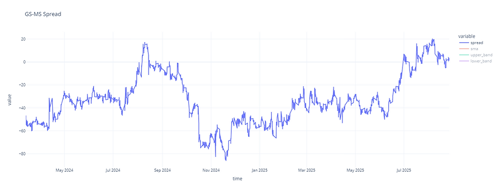
Looking at the spread chart, we can see that the spread ranges between -80 and +20. Also, there are periods where the consolidation is very evident which is optimal for statistical arbitrage.
Step 3 - Calculate Indicators
In order to identify buy and sell levels, we will use the Bollinger Bands indicator which is commonly used for mean reversion strategies.
Indicator Values:
Timeframe: 1 hour
Period: 40
Number of Standard Deviations: 1.75
Using the code below, we are computing Bollinger Bands with pandas library
spread_df['sma'] = spread_df['spread'].rolling(8 * 5).mean()
spread_df['std'] = spread_df['spread'].rolling(8 * 5).std()

spread_df['upper_band'] = spread_df['sma'] + spread_df['std'] * 1.75
spread_df['lower_band'] = spread_df['sma'] - spread_df['std'] * 1.75
By plotting the indicators, we get the following chart:
px.line(spread_df, x='time', y=['spread', 'sma', 'upper_band', 'lower_band'], title='GS-MS Spread')
Step 4 - Backtest the Trading Strategy
In this section, I will show you the trading logic and how to run a backtest on the chart above.
Trading Logic
Entry:
Whenever the spread crosses below the lower_band, we buy.
Whenever the spread crosses above the upper_band, we sell.
Note: Buying the spread represents buying 1 unit of GS and selling 5 units of MS and vice versa
Exit:
Once a position is open, we exit buy positions when spread is above sma.
We exit sell positions when spread is below sma.
Using our backtesting class, we can write it in code as below:
def on_bar(bt, data, strategy_params):

    symbol = 'gs_ms_statarb'

    num_open_positions = bt.get_num_open_positions()

    # entry
    if data['spread'] < data['lower_band'] and num_open_positions == 0:
        bt.open_trade(symbol, 'buy', 100)

    if data['spread'] > data['upper_band'] and num_open_positions == 0:
        bt.open_trade(symbol, 'sell', 100)

    # exit
    if data['spread'] < data['sma'] and num_open_positions > 0:
        bt.close_trades(action='sell')

    if data['spread'] > data['sma'] and num_open_positions > 0:
        bt.close_trades(action='buy')
Once the strategy logic is defined, we just need to initialize our backtester class and input some backtest parameters.
Parameters:
The commission represents the transaction costs and the bid-ask spread is also included in the commission.
Commission: -0.5 USD / unit
Running the backtest
In the code block below, we are running our backtest which then generates trades.
# initialize backtesting class
bt = Backtester(commission=-0.5)

bt.set_strategy(on_bar)
bt.set_historical_data(spread_df)

bt.run()

trades_df = pd.DataFrame.from_dict(bt.trades, orient='index')
trades_df
Visualizing the backtest
Now that the trades are generated, we can vizualize the Cumulative PnL and the Trades on a chart using the code below:
trades_df['cumulative_profit'] = trades_df['net_profit'].cumsum()
pnl_fig = px.line(trades_df, x='open_time', y=['cumulative_profit'], width=1200, title='Cumulative PnL')

pnl_fig
bt.visualize_backtest(indicators=['sma', 'upper_band', 'lower_band'])Download Jupyter Notebook and Trading Bot Template
In the link below you can download the my Jupyter Notebook and my Trading Bot Template for statistical arbitrage.
Risk Warning
The following code only represents the general framework of our strategies and may not be suitable for live trading on their own.
The script contains automated trading features. Please make sure that you understand the risks of automated trading. It is strongly recommended that you test your code on a Paper Trading account before going live.
The strategies showcased in our Youtube videos may contain additional modifications and different execution algorithms and may therefore have a different trading result. The strategy parameters and rules may change over time due to different market conditions.
Past performance is not an indicator of future results. By trading this strategy you are at risk of losing your money.
Content is educational only and does not serve as investment advice.
ATJ Traders is not responsible for any losses generated from the scripts provided.
Comments